Lesson 3 Predictive Regression Part I
3.1 Introduction
This is the first of two lessons that will teach you how to implement and interpret predictive linear regression in R. For the moment we won't worry about causality and we won't talk about heteroskedasticity or autocorrelation. In this first lesson, we'll introduce the basics using a simple dataset that you can download from my website and display as follows:
library(readr)
kids <- read_csv("http://ditraglia.com/data/child_test_data.csv")
kids
## # A tibble: 434 × 4
## kid.score mom.hs mom.iq mom.age
## <dbl> <dbl> <dbl> <dbl>
## 1 65 1 121. 27
## 2 98 1 89.4 25
## 3 85 1 115. 27
## 4 83 1 99.4 25
## 5 115 1 92.7 27
## 6 98 0 108. 18
## 7 69 1 139. 20
## 8 106 1 125. 23
## 9 102 1 81.6 24
## 10 95 1 95.1 19
## # … with 424 more rowsEach row of the tibble kids contains information on a three-year old child. The first column gives the child's test score at age three, while the remaining columns provide information about each child's mother:
kid.scorechild test score at age 3mom.ageage of mother at birth of childmom.hsmother completed high school? (1 = yes)mom.iqmother's IQ score
The columns kid.score gives the child's test score at age three. The remaining columns describe the child's mother: mom.age is mother's age at the birth of the child, mom.hs is a dummy variable that equals one the mother completed high school, and mom.iq is the mother's IQ score. Our main goal will be to predict a child's test score based on mother characteristics. But stay alert: in some of the exercises I may be a bit devious and ask you to predict something else!
3.1.1 Exercise
Using a dot . to separate words in a variable name isn't great coding style: it's better to use an underscore _. Search the dplyr help files for the command rename() and then use this command to replace each instance of a . in the column names of kids with an underscore _.
library(dplyr)
kids <- kids %>%
  rename(kid_score = kid.score,
         mom_hs = mom.hs,
         mom_iq = mom.iq,
         mom_age = mom.age)
3.2 The Least Squares Problem
Suppose we observe a dataset with \(n\) observations \((Y_i, X_i)\) where \(Y_i\) is an outcome variable for person \(i\)--the thing we want to predict--and \(X_i\) is a vector of \(p\) predictor variables--the things we'll use to make our prediction. In the kids dataset, our outcome is kid_score and our predictors are mom_hs, mom_age, and mom_iq. Our goal is to build a model of the form \(X'\beta = \sum_{j=1}^p \beta_j X_{j}\) that we can use to predict \(Y\) for a person who is not in our dataset. The constants \(\beta_j\) are called coefficients and a model of this form is called a linear model because the \(\beta_j\) enter linearly: they're not raised to any powers etc. Ordinary least squares (OLS) uses the observed data to find the coefficients \(\widehat{\beta}\) that solve the least squares problem
\[
\underset{\beta}{\text{minimize}} \sum_{i=1}^n (Y_i - X_i'\beta)^2.
\]
In case you were wondering "but wait, where's the intercept?" I should point out that some people prefer to write \((Y_i - \beta_0 - X_i' \beta)\) rather than \((Y_i - X_i'\beta)\). To allow an intercept using my notation, simply treat the first element of my \(X_i\) vector as a \(1\) and the first element of my \(\beta\) vector as the intercept.
3.2.1 Exercise
Suppose we want to regress the outcome \(Y_i\) on an intercept only, in other words we want to minimize \(\sum_{i=1}^n (Y_i - \beta)^2\) over \(\beta\). What is the solution? Does this make sense?
Differentiating with respect to \(\beta\), the first order condition is \(-2 \sum_{i=1}^n (Y_i - \widehat{\beta}) = 0\). Because the objective function is convex, this characterizes the global minimum. Re-arranging and solving for \(\widehat{\beta}\) gives \(\widehat{\beta} = \frac{1}{n}\sum_{i=1}^n Y_i\). In other words \(\widehat{\beta} = \bar{Y}\), the sample mean. This makes sense: the sample mean is a reasonable prediction of the next \(Y\)-observation if you have no other information to work with. Here we've shown that it is also the least squares solution.
3.3 Linear Regression with lm()
The R function lm(), short for linear model, solves the least squares problem. Its basic syntax is lm([formula], [dataframe]) where [formula] is an R formula--an object that describes the regression we want to run--and [dataframe] is the name of a data frame containing our \(X\) and \(Y\) observations, e.g. kids. R formulas can be a bit confusing when you first encounter them, so I'll explain the details in stages. For the moment, there are two symbols you need to learn: ~ and +
The tilde symbol ~ is used to separate the "left hand side" and "right hand side" of a formula: the outcome goes on the left of the ~ and the predictors go on the right. For example, to regress kid_score on mom_iq we use the command
lm(kid_score ~ mom_iq, kids)##
## Call:
## lm(formula = kid_score ~ mom_iq, data = kids)
##
## Coefficients:
## (Intercept) mom_iq
## 25.80 0.61This tells R: "please solve the least squares problem to predict kid_score using mom_iq based on the data contained in kids." Notice that R includes an intercept in the regression automatically. This is a good default, because it seldom makes sense to run a regression without an intercept. When you want to run a regression with multiple right-hand side predictors, use the plus sign + to separate them. For example, to regress kid_score on mom_iq and mom_ageuse the command
lm(kid_score ~ mom_iq + mom_age, kids)##
## Call:
## lm(formula = kid_score ~ mom_iq + mom_age, data = kids)
##
## Coefficients:
## (Intercept) mom_iq mom_age
## 17.5962 0.6036 0.38813.3.1 Exercise
- Interpret the regression coefficients from
lm(kid_score ~ mom_iq, kids).
Consider two kids whose mothers differ by 1 point in mom_iq. We would predict that the kid whose mom has the higher value of mom_iq will score about 0.6 points higher in kid_score.
lm(kid_score ~ mom_iq, kids)##
## Call:
## lm(formula = kid_score ~ mom_iq, data = kids)
##
## Coefficients:
## (Intercept) mom_iq
## 25.80 0.61- Run a linear regression to predict
mom_hsusingkid_scoreandmom_iq.
lm(mom_hs ~ kid_score + mom_iq, kids)##
## Call:
## lm(formula = mom_hs ~ kid_score + mom_iq, data = kids)
##
## Coefficients:
## (Intercept) kid_score mom_iq
## -0.060135 0.002775 0.0060503.4 Plotting the Regression Line
The ggplot2 package makes it easy to produce an attractive and informative plot of the results of a simple linear regression. Using what we learned in our last lesson, we know how to make a scatter plot of mom_iq and kid_score:
library(ggplot2)
ggplot(kids) +
  geom_point(aes(x = mom_iq, y = kid_score))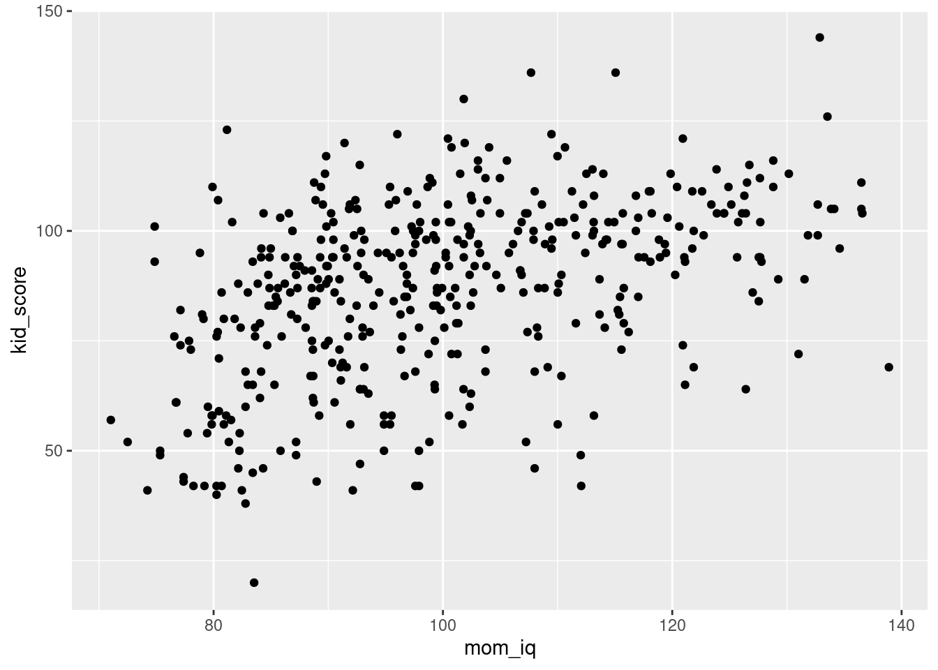
To add the regression line, we'll use geom_smooth(), a function for plotting smoothed conditional means. We can use geom_smooth() in exactly the same way as geom_point() by specifying aes() to set the x and y variables. By default, geom_smooth() plots a non-parametric regression curve rather than a linear regression:
ggplot(kids) +
  geom_point(aes(x = mom_iq, y = kid_score)) +
  geom_smooth(aes(x = mom_iq, y = kid_score))
## `geom_smooth()` using method = 'loess' and formula 'y ~ x'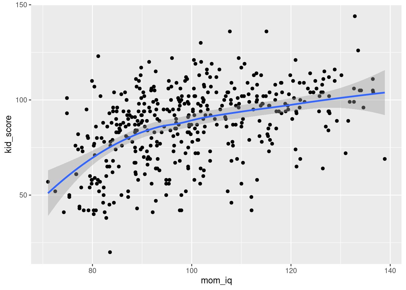
Notice that we had to type aes(x = mom_iq, y = kid_score) twice in the preceding code chunk. This is tedious and error-prone. In more complicated plots that contain multiple geom functions, life is much simpler if we specify our desired aes() once. To do this, pass it as an argument to ggplot rather than to the geom, for example
ggplot(kids, aes(x = mom_iq, y = kid_score)) +
  geom_point() +
  geom_smooth()
To plot a regression line rather than this non-parametric regression function, we merely need to set method = 'lm in geom_smooth(), for example
ggplot(kids, aes(x = mom_iq, y = kid_score)) +
  geom_point() +
geom_smooth(method = 'lm') 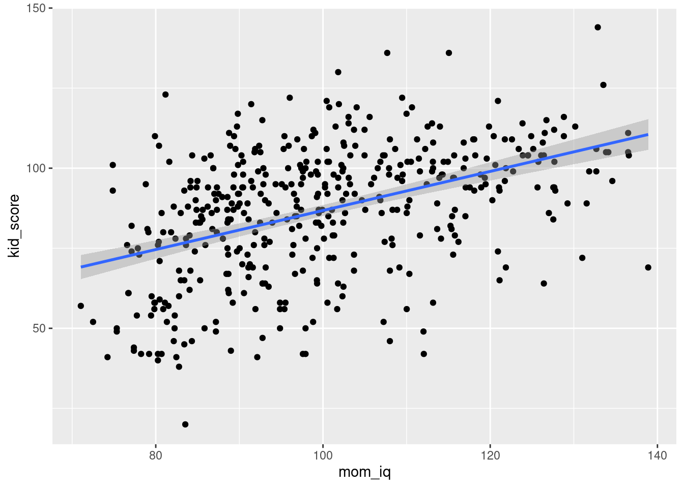
By default this plots the regression line from the regression y ~ x.
3.4.1 Exercise
- Use
ggplot()to make a scatter plot withmom_ageon the horizontal axis andkid_scoreon the vertical axis.
ggplot(kids, aes(x = mom_age, y = kid_score)) +
  geom_point()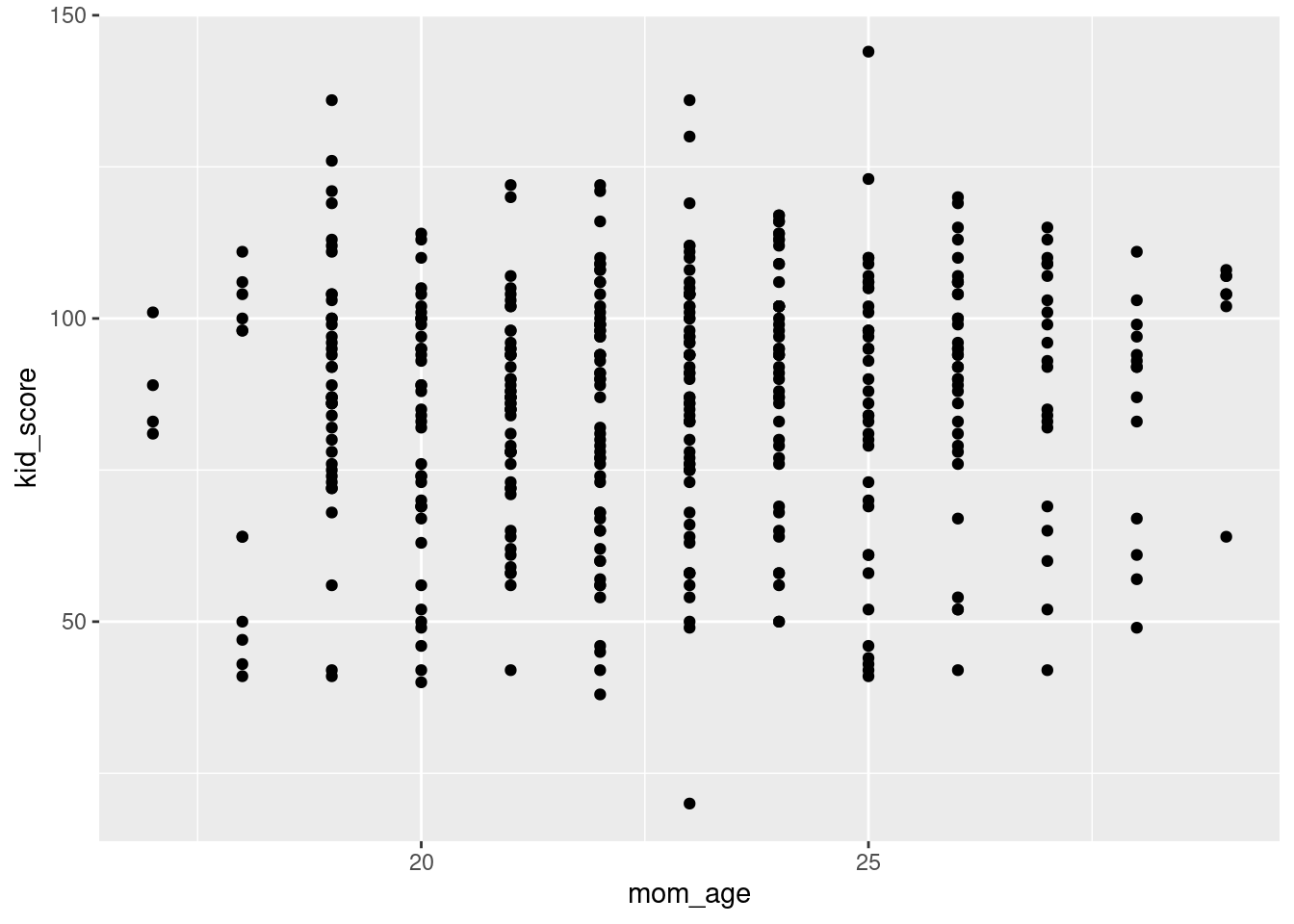
- Use
geom_smooth()to including the non-parametric regression function on the preceding plot.
ggplot(kids, aes(x = mom_age, y = kid_score)) +
  geom_point() +
  geom_smooth()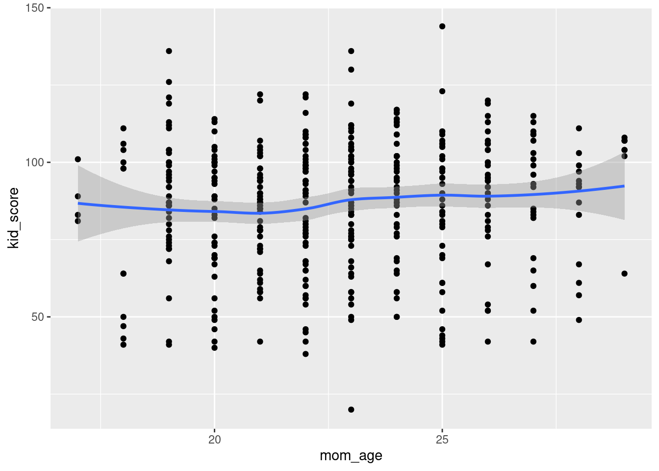
- Modify the preceding to include the regression line corresponding to
kid_score ~ mom_ageon the scatter plot rather than the non-parametric regression function.
ggplot(kids, aes(x = mom_age, y = kid_score)) +
  geom_point() +
  geom_smooth(method = 'lm')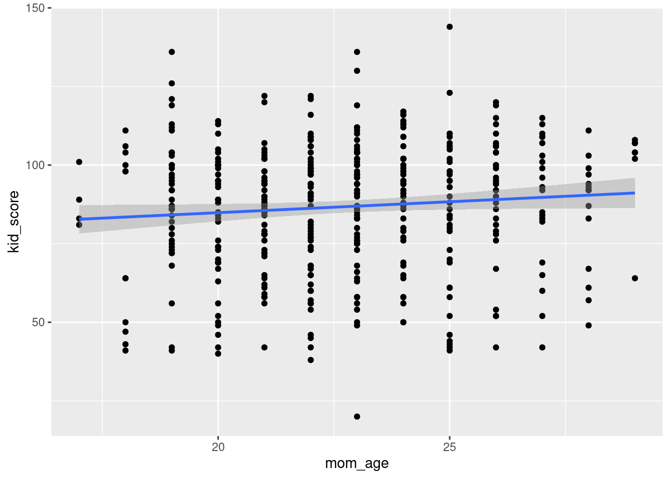
3.5 Getting More from lm()
If we simply run lm as above, R will display only the estimated regression coefficients and the command that we used to run the regression: Call.
To get more information, we need to store the results of our regression using the assignment operator <- for example:
reg1 <- lm(kid_score ~ mom_iq, kids)If you run the preceding line of code in the R console, it won't produce any output. But if you check your R environment after running it, you'll see a new List object: reg1. To see what's inside this list, we can use the command str:
str(reg1)## List of 12
## $ coefficients : Named num [1:2] 25.8 0.61
## ..- attr(*, "names")= chr [1:2] "(Intercept)" "mom_iq"
## $ residuals : Named num [1:434] -34.68 17.69 -11.22 -3.46 32.63 ...
## ..- attr(*, "names")= chr [1:434] "1" "2" "3" "4" ...
## $ effects : Named num [1:434] -1808.22 190.39 -8.77 -1.96 33.73 ...
## ..- attr(*, "names")= chr [1:434] "(Intercept)" "mom_iq" "" "" ...
## $ rank : int 2
## $ fitted.values: Named num [1:434] 99.7 80.3 96.2 86.5 82.4 ...
## ..- attr(*, "names")= chr [1:434] "1" "2" "3" "4" ...
....Don't panic: you don't need to know what all of these list elements are.
The important thing to understand is that lm returns a list from which we can extract important information about the regression we have run.
To extract the regression coefficient estimates, we use the function coefficients() or coef() for short
coef(reg1)## (Intercept) mom_iq
## 25.7997778 0.6099746To extract the regression residuals, we use the function residuals() or resid() for short
resid(reg1)## 1 2 3 4 5 6
## -34.67839049 17.69174662 -11.21717291 -3.46152907 32.62769741 6.38284487
## 7 8 9 10 11 12
## -41.52104074 3.86488149 26.41438662 11.20806784 11.17050590 -25.66178773
## 13 14 15 16 17 18
## 3.93517580 -17.40659730 14.87699469 10.74760539 6.40273692 5.13172163
## 19 20 21 22 23 24
## -2.44440289 15.87116678 9.04396998 11.90180808 14.47664178 0.24807074
## 25 26 27 28 29 30
## 13.66974891 -4.06297022 -14.03359486 -7.52559318 2.18354609 2.47533381
....To extract the fitted values i.e. \(\hat{Y}_i \equiv X_i'\hat{\beta}\), the predicted values of, we use fitted.values
fitted.values(reg1)## 1 2 3 4 5 6 7 8
## 99.67839 80.30825 96.21717 86.46153 82.37230 91.61716 110.52104 102.13512
## 9 10 11 12 13 14 15 16
## 75.58561 83.79193 79.82949 83.66179 80.06482 95.40660 87.12301 99.25239
## 17 18 19 20 21 22 23 24
## 95.59726 93.86828 107.44440 85.12883 92.95603 103.09819 85.52336 86.75193
## 25 26 27 28 29 30 31 32
## 85.33025 100.06297 86.03359 85.52559 74.81645 95.52467 92.37138 87.90567
## 33 34 35 36 37 38 39 40
## 97.75549 92.06345 84.67978 82.44896 84.29520 91.07649 78.98774 80.30825
....3.5.1 Exercise
- Plot a histogram of the residuals from
reg1usingggplotwith a bin width of 5. Is there anything noteworthy about this plot?
There seems to be a bit of left skewness in the residuals.
library(ggplot2)
ggplot() +
  geom_histogram(aes(x = resid(reg1)), binwidth = 5)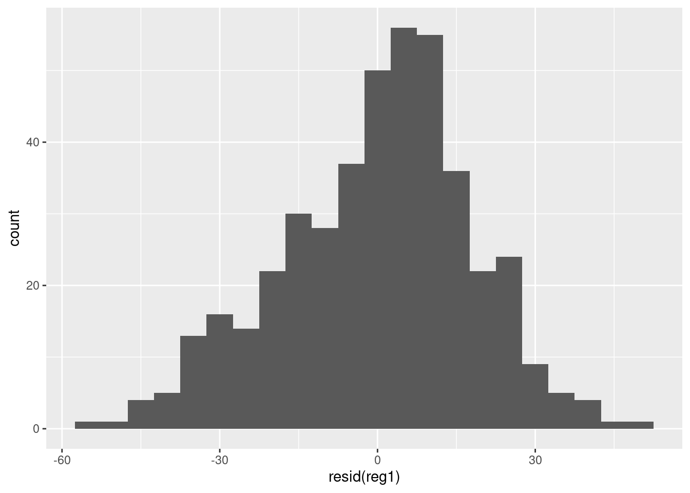
- Calculate the residuals "by hand" by subtracting the fitted values from
reg1from the columnkid_scoreinkids. Use the R functionall.equalto check that this gives the same result asresid().
They give exactly the same result:
all.equal(resid(reg1), kids$kid_score - fitted.values(reg1))## [1] TRUE- As long as you include an intercept in your regression, the residuals will sum to zero. Verify that this is true (up to machine precision!) of the residuals from
reg1
Close enough!
sum(resid(reg1))## [1] 1.056155e-12- By construction, the regression residuals are uncorrelated with any predictors included in the regression. Verify that this holds (up to machine precision!) for
reg1.
Again, close enough!
cor(resid(reg1), kids$mom_iq)## [1] 3.121525e-163.6 Summarizing The Ouput of lm()
To view the "usual" summary of regression output, we use the summary() function:
summary(reg1)##
## Call:
## lm(formula = kid_score ~ mom_iq, data = kids)
##
## Residuals:
## Min 1Q Median 3Q Max
## -56.753 -12.074 2.217 11.710 47.691
##
## Coefficients:
## Estimate Std. Error t value Pr(>|t|)
## (Intercept) 25.79978 5.91741 4.36 1.63e-05 ***
## mom_iq 0.60997 0.05852 10.42 < 2e-16 ***
## ---
## Signif. codes: 0 '***' 0.001 '**' 0.01 '*' 0.05 '.' 0.1 ' ' 1
##
## Residual standard error: 18.27 on 432 degrees of freedom
## Multiple R-squared: 0.201, Adjusted R-squared: 0.1991
## F-statistic: 108.6 on 1 and 432 DF, p-value: < 2.2e-16Among other things, summary shows us the coefficient estimates and associated standard errors for each regressor. It also displays the t-value (Estimate / SE) and associated p-value for a test of the null hypothesis \(H_0\colon \beta = 0\) versus \(H_1\colon \beta \neq 0\). Farther down in the output, summary provides the residual standard error, the R-squared, and the F-statistic and associated p-value for a test of the null hypothesis that all regression coefficients except for the intercept are zero.10
Health warning: by default, lm() computes standard errors and p-values under the classical regression assumptions. In particular, unless you explicitly tell R to do otherwise, it will assume that the regression errors \(\varepsilon_i \equiv Y_i - X_i' \beta\) are homoskedastic, and iid. If you're not quite sure what this means, or if you're worried that I'm sweeping important details under the rug, fear not: we'll revisit this in a later lesson. For the moment, let me offer you the following mantra, paraphrasing the wisdom of my favorite professor from grad school:
You can always run a [predictive] linear regression; it's inference that requires assumptions.
3.6.1 Exercise
Use the kids tibble to run a regression that uses kid_score and mom_hs to predict mom_iq. Store your results in an object called reg_reverse and then display a summary of the regression results.
reg_reverse <- lm(mom_iq ~ mom_hs + kid_score, kids)
summary(reg_reverse)
##
## Call:
## lm(formula = mom_iq ~ mom_hs + kid_score, data = kids)
##
## Residuals:
## Min 1Q Median 3Q Max
## -31.046 -10.412 -1.762 8.839 42.714
##
## Coefficients:
## Estimate Std. Error t value Pr(>|t|)
## (Intercept) 68.86638 2.82454 24.381 < 2e-16 ***
## mom_hs 6.82821 1.58450 4.309 2.03e-05 ***
## kid_score 0.29688 0.03189 9.309 < 2e-16 ***
## ---
## Signif. codes: 0 '***' 0.001 '**' 0.01 '*' 0.05 '.' 0.1 ' ' 1
##
## Residual standard error: 13.16 on 431 degrees of freedom
## Multiple R-squared: 0.234, Adjusted R-squared: 0.2304
## F-statistic: 65.82 on 2 and 431 DF, p-value: < 2.2e-163.7 Tidying up with broom
We saw above that lm() returns a list. It turns out that summary(), when applied to an lm() object, also returns a list:
str(summary(reg1))## List of 11
## $ call : language lm(formula = kid_score ~ mom_iq, data = kids)
## $ terms :Classes 'terms', 'formula' language kid_score ~ mom_iq
## .. ..- attr(*, "variables")= language list(kid_score, mom_iq)
## .. ..- attr(*, "factors")= int [1:2, 1] 0 1
## .. .. ..- attr(*, "dimnames")=List of 2
## .. .. .. ..$ : chr [1:2] "kid_score" "mom_iq"
## .. .. .. ..$ : chr "mom_iq"
## .. ..- attr(*, "term.labels")= chr "mom_iq"
## .. ..- attr(*, "order")= int 1
....In principle, this gives us a way of extracting particular pieces of information from a table of regression output generated by summary(). For example, if you carefully examine the output of str(summary(reg1)) you'll find a named list element called r.squared. By accessing this element, you can pluck out the R-squared from summary(reg1) as follows:
summary(reg1)$r.squared## [1] 0.2009512Similarly, you could extract F-statistics and associated degrees of freedom by accessing You could extract the information
That wasn't so bad! But now suppose you wanted to extract the estimates, standard errors, and p-values from reg1. While it's possible to do this by poring over the output of str(summary(reg1)), there's a much easier way.
The broom package provides some extremely useful functions for extracting regression output. Best of all, the same tools apply to models that we'll meet in later lessons. Use tidy() to create a tibble containing regression estimates, standard errors, t-statistics, and p-values e.g.
library(broom)
tidy(reg1)
## # A tibble: 2 × 5
## term estimate std.error statistic p.value
## <chr> <dbl> <dbl> <dbl> <dbl>
## 1 (Intercept) 25.8 5.92 4.36 1.63e- 5
## 2 mom_iq 0.610 0.0585 10.4 7.66e-23Use glance() to create a tibble that summarizes various measures of model fit:
glance(reg1)## # A tibble: 1 × 12
## r.squared adj.r.squared sigma statistic p.value df logLik AIC BIC
## <dbl> <dbl> <dbl> <dbl> <dbl> <dbl> <dbl> <dbl> <dbl>
## 1 0.201 0.199 18.3 109. 7.66e-23 1 -1876. 3757. 3769.
## # … with 3 more variables: deviance <dbl>, df.residual <int>, nobs <int>Finally, use augment() to create a tibble that merges the tibble you used to run your regression with the corresponding regression fitted values, residuals, etc.
augment(reg1, kids)## # A tibble: 434 × 10
## kid_score mom_hs mom_iq mom_age .fitted .resid .hat .sigma .cooksd
## <dbl> <dbl> <dbl> <dbl> <dbl> <dbl> <dbl> <dbl> <dbl>
## 1 65 1 121. 27 99.7 -34.7 0.00688 18.2 0.0126
## 2 98 1 89.4 25 80.3 17.7 0.00347 18.3 0.00164
## 3 85 1 115. 27 96.2 -11.2 0.00475 18.3 0.000905
## 4 83 1 99.4 25 86.5 -3.46 0.00231 18.3 0.0000416
## 5 115 1 92.7 27 82.4 32.6 0.00284 18.2 0.00456
## 6 98 0 108. 18 91.6 6.38 0.00295 18.3 0.000181
## 7 69 1 139. 20 111. -41.5 0.0178 18.2 0.0478
## 8 106 1 125. 23 102. 3.86 0.00879 18.3 0.000200
## 9 102 1 81.6 24 75.6 26.4 0.00577 18.2 0.00611
## 10 95 1 95.1 19 83.8 11.2 0.00255 18.3 0.000483
## # … with 424 more rows, and 1 more variable: .std.resid <dbl>Notice that augment() uses a dot "." to begin the name of any column that it merges. This avoids potential clashes with columns you already have in your dataset. After all, you'd never start a column name with a dot would you?
3.7.1 Exercise
To answer the following, you may need to consult the help files for tidy.lm(), glance.lm(), and augment.lm() from the broom package.
- Use
dplyrandtidy()to display the regression estimate, standard error, t-statistic, and p-value for the predictorkid_scoreinreg_reversefrom above.
reg_reverse %>%
  tidy() %>%
  filter(term == 'kid_score')
## # A tibble: 1 × 5
## term estimate std.error statistic p.value
## <chr> <dbl> <dbl> <dbl> <dbl>
## 1 kid_score 0.297 0.0319 9.31 6.61e-19- Use
ggplot()andaugment()to make a scatterplot with the fitted values fromreg_reverseon the horizontal axis andmom_iqon the vertical axis. Usegeom_abline()to add a 45-degree line to your plot. (You may need to read the help file for this function.)
augment(reg_reverse, kids) %>%
  ggplot(aes(x = .fitted, y = mom_iq)) +
  geom_point() +
  geom_abline(intercept = 0, slope = 1)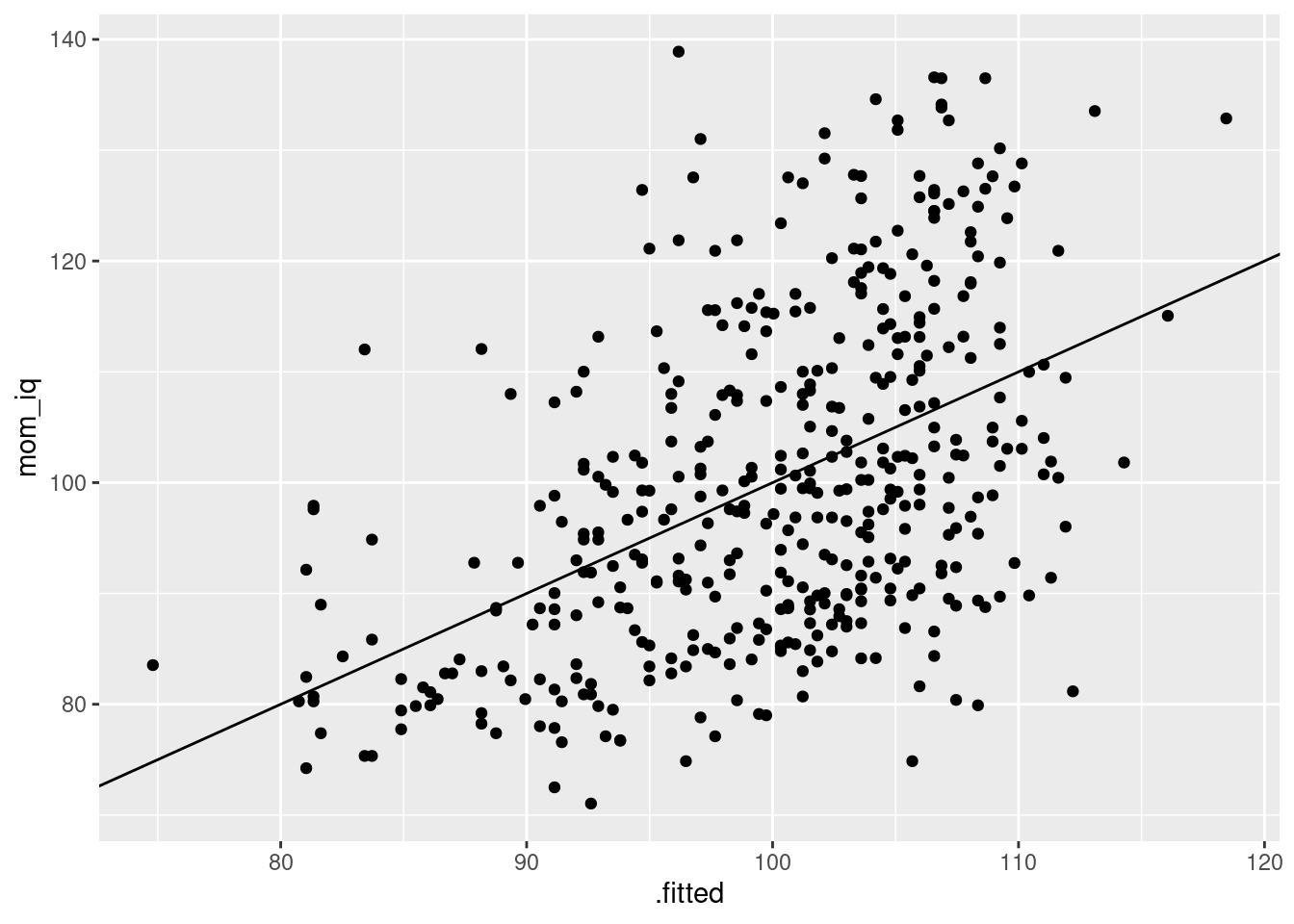
- Continuing from the preceding exercise, run a regression of
mom_iqon the fitted values fromreg_reverseand display the estimated regression coefficients. Compare the R-squared of this regression to that ofreg_reverse. Explain your results.
When we regress \(Y_i\) on \(\widehat{Y}_i\), the fitted values from a regression of \(Y_i\) on \(X_i\), we get an intercept of zero and a slope of one:
kids_augmented <- augment(reg_reverse, kids)
reg_y_vs_fitted <- lm(mom_iq ~ .fitted, kids_augmented)
tidy(reg_y_vs_fitted)
## # A tibble: 2 × 5
## term estimate std.error statistic p.value
## <chr> <dbl> <dbl> <dbl> <dbl>
## 1 (Intercept) 1.96e-13 8.73 2.25e-14 1.00e+ 0
## 2 .fitted 1.00e+ 0 0.0871 1.15e+ 1 7.85e-27This makes sense. Suppose we wanted to choose \(\alpha_0\) and \(\alpha_1\) to minimize \(\sum_{i=1}^n (Y_i - \alpha_0 - \alpha_1 \widehat{Y}_i)^2\) where \(\widehat{Y}_i = \widehat{\beta}_0 + X_i'\widehat{\beta}_1\). This is equivalent to minimizing \[ \sum_{i=1}^n \left[Y_i - (\alpha_0 + \widehat{\beta}_0) - X_i'(\alpha_1\widehat{\beta}_1)\right]^2. \] By construction \(\widehat{\beta}_0\) and \(\widehat{\beta}_1\) minimize \(\sum_{i=1}^n (Y_i - \beta_0 - X_i'\beta_1)^2\), so unless \(\widehat{\alpha_0} = 0\) and \(\widehat{\alpha_1} = 1\) we'd have a contradiction! Similar reasoning explains why the R-squared values for the two regressions are the same:
c(glance(reg_reverse)$r.squared, glance(reg_y_vs_fitted)$r.squared)## [1] 0.2339581 0.2339581The R-squared of a regression equals \(1 - \text{SS}_{\text{residual}} / \text{SS}_{\text{total}}\) \[ \text{SS}_{\text{total}} = \sum_{i=1}^n (Y_i - \bar{Y})^2,\quad \text{SS}_{\text{residual}} = \sum_{i=1}^n (Y_i - \widehat{Y}_i^2) \] The total sum of squares is the same for both regressions because they have the same outcome variable. The residual sum of squares is the same because \(\widehat{\alpha}_0 = 0\) and \(\widehat{\alpha}_1 = 1\) together imply that both regressions have the same fitted values.
3.8 Dummy Variables with lm()
The column mom_hs in kids is a dummy variable, also known as a binary variable. It equals 1 if a child's mother graduated from college and 0 otherwise. For this reason, the coefficient on mom_hs in the following regression tells us the difference of mean test scores between kids whose mothers graduated from college and those whose mothers did not, while the intercept tells us the mean of kid_score for children whose mothers didn't graduate from high school:
lm(kid_score ~ mom_hs, kids)##
## Call:
## lm(formula = kid_score ~ mom_hs, data = kids)
##
## Coefficients:
## (Intercept) mom_hs
## 77.55 11.77Although it's represented using the numerical values 0 and 1, mom_hs doesn't actually encode quantitative information. The numerical values are just shorthand for two different categories: mom_hs is a categorical variable. To keep from getting confused, it's good practice to make categorical variables obvious by storing them as character or factor data. Here I create a new column, mom_education, that stores the same information as mom_hs as a factor:
kids <- kids %>%
  mutate(mom_education = if_else(mom_hs == 1, 'High School', 'No High School')) %>%
  mutate(mom_education = factor(mom_education, levels = unique(mom_education)))
The column mom_education is a factor, R's built-in representation of a categorical variable. So what happens if we include mom_education in our regression in place of mom_hs?
lm(kid_score ~ mom_education, kids)##
## Call:
## lm(formula = kid_score ~ mom_education, data = kids)
##
## Coefficients:
## (Intercept) mom_educationNo High School
## 89.32 -11.77Wait a minute; now the estimate is negative! We can't run a regression that includes an intercept and a coefficient for each level of a dummy variable--this is the dummy variable trap!--so R has excluded one of them. Rather capriciously, lm() has chosen to treat High School as the omitted category.
We can override this behavior by using fct_relevel() from the forcats package. The following code tells R that we want 'No High School' to be the first ordered factor level, the level that lm() treats as the omitted category by default:
library(forcats)
kids <- kids %>%
  mutate(mom_education = fct_relevel(mom_education, 'No High School'))
lm(kid_score ~ mom_education, kids)
##
## Call:
## lm(formula = kid_score ~ mom_education, data = kids)
##
## Coefficients:
## (Intercept) mom_educationHigh School
## 77.55 11.77In the exercise you'll explore how lm() handles categorical variables that take on more than two values. In your econometrics class you probably learned that we can use two dummy variables to encode a three-valued categorical variable, four dummy variables to encode a four-valued categorical variable, and so on. You may wonder if we need to explicitly construct these dummy variables in R. The answer is no: lm() handles things for us automatically, as you're about to discover. This is worth putting in bold: you don't have to explicitly construct dummy variables in R. The lm() function will construct them for you.
3.8.1 Exercise
- Read the help file for the base R function
cut(). Setting the argumentbreakstoc(16, 19, 23, 26, 29), use this function in concert withdplyr()to create a factor variable calledmom_age_binstokids. Use the base R functionlevels()to display the factor levels ofmom_age_bins.
kids <- kids %>%
  mutate(mom_age_bins = cut(mom_age, c(16, 19, 23, 26, 29)))
levels(kids$mom_age_bins)
## [1] "(16,19]" "(19,23]" "(23,26]" "(26,29]"- Run a linear regression of
kid_scoreonmom_age_binsand display the coefficients. Explain the results.
R "expands" the factor variable mom_age_bins into a collection of dummy variables before running the regression. It names these dummies in an obvious way based on the levels that mom_age_bins takes on:
lm(kid_score ~ mom_age_bins, kids)##
## Call:
## lm(formula = kid_score ~ mom_age_bins, data = kids)
##
## Coefficients:
## (Intercept) mom_age_bins(19,23] mom_age_bins(23,26]
## 87.054 -2.308 2.293
## mom_age_bins(26,29]
## 2.232In words: R has run a regression of kid_score on a constant (the intercept), a dummy for mother's age in the range (19,23], a dummy for mother's age in the range (23,26] and a dummy for mother's age in the range (26,29].
From running levels(kids$mom_age_bins) above, we know this means the omitted category is (16,19]. This corresponds to the intercept in the regression, so the average value of kid_score for a child whose mother's age lies in the range (16,19] is around 87 points. All the other coefficients are differences of means relative to this category of "teen moms." For example, kids whose mothers' age is in the range (19,23] score about two points lower, on average, then kids whose mothers' age is in the range (16,19].
- Re-run the preceding regression, but use
fct_relevel()from theforcatspackage make(26,29]the omitted category formom_age_bins.
kids <- kids %>%
  mutate(mom_age_bins = fct_relevel(mom_age_bins, '(26,29]'))
lm(kid_score ~ mom_age_bins, kids)
##
## Call:
## lm(formula = kid_score ~ mom_age_bins, data = kids)
##
## Coefficients:
## (Intercept) mom_age_bins(16,19] mom_age_bins(19,23]
## 89.28571 -2.23214 -4.54043
## mom_age_bins(23,26]
## 0.061063.9 Fun with R Formulas
It's time to learn some more about R formulas. But before we do, you may ask "why bother?" It's true that you run just about any regression you need using nothing more complicated than + and ~ as introduced above. I know, because I did this for the better part of a decade! But a key goal of this book is showing you how to work smarter rather than harder, both to make your own life easier and help others replicate your work. If you ever plan to fit more than a handful of models with more than a handful of variables, it's worth your time to learn about formulas. You've already met the special symbols ~ and + explained in the following table. In the next few sub-sections, I'll walk you through the others: ., -, 1, :, *, ^, and I().
| Symbol | Purpose | Example | In Words |
|---|---|---|---|
~ |
separate LHS and RHS of formula | y ~ x |
regress y on x |
+ |
add variable to a formula | y ~ x + z |
regress y on x and z |
. |
denotes "everything else" | y ~ . |
regress y on all other variables in a data frame |
- |
remove variable from a formula | y ~ . - x |
regress y on all other variables except z |
1 |
denotes intercept | y ~ x - 1 |
regress y on x without an intercept |
: |
construct interaction term | y ~ x + z + x:z |
regress y on x, z, and the product x times z |
* |
shorthand for levels plus interaction | y ~ x * z |
regress y on x, z, and the product x times z |
^ |
higher order interactions | y ~ (x + z + w)^3 |
regress y on x, z, w, all two-way interactions, and the three-way interactions |
I() |
"as-is" - override special meanings of other symbols from this table | y ~ x + I(x^2) |
regress y on x and x squared |
3.9.1 "Everything Else" - The Dot .
Sometimes all you want to do is run a regression of one variable on everything else. If you have lots of predictors, typing out all of their names, each separated by a + sign, is painful and error-prone. Fortunately there's a shortcut: the dot .
lm(kid_score ~ ., kids)##
## Call:
## lm(formula = kid_score ~ ., data = kids)
##
## Coefficients:
## (Intercept) mom_hs mom_iq
## -8.571 5.638 0.571
## mom_age mom_educationHigh School mom_age_bins(16,19]
## 1.155 NA 14.048
## mom_age_bins(19,23] mom_age_bins(23,26]
## 7.205 7.631This command tells R to regress kid_score on everything else in kids. Notice that the coefficient mom_educationHigh School is NA, in other words missing. This is because you can't run a regression on mom_hs and mom_education at the same time: they're two versions of exactly the same information and hence are perfectly co-linear, so R drops one of them.
We'll encounter the dot in many guises later in this lesson and elsewhere. Wherever you see it, replace it mentally with the word "everything" and you'll never be confused. The rest will be clear from context.
3.9.2 Removing Predictors with -
The regression we ran above using the dot . was very silly: it included both mom_hs and mom_education, and it also included both mom_age_bins and mom_age. Suppose we wanted to run a regression of kid_score on everything except mom_age_bins and mom_education. This is easy to achieve using the minus sign - as follows:
lm(kid_score ~ . - mom_age_bins - mom_education, kids)##
## Call:
## lm(formula = kid_score ~ . - mom_age_bins - mom_education, data = kids)
##
## Coefficients:
## (Intercept) mom_hs mom_iq mom_age
## 20.9847 5.6472 0.5625 0.2248Think of + as saying "add me to the regression" and - as saying "remove me from the regression." This use of - is very similar to what you've seen in the select() function from dplyr. And as in dplyr, we can use it to remove one variable or more than one.
3.9.3 The Intercept: 1
It almost always makes sense to include an intercept when you run a linear regression. Without one, we're forced to predict that \(Y\) will be zero when \(X\) is zero. Because this is usually a bad idea, lm() includes an intercept by default:
lm(kid_score ~ mom_iq, kids)##
## Call:
## lm(formula = kid_score ~ mom_iq, data = kids)
##
## Coefficients:
## (Intercept) mom_iq
## 25.80 0.61In some special cases, however, we may have a reason to run a regression without an intercept. R's formula syntax denotes the intercept by 1. Armed with this knowledge, we can remove it from our regression using - as introduced above:
lm(kid_score ~ mom_iq - 1, kids)##
## Call:
## lm(formula = kid_score ~ mom_iq - 1, data = kids)
##
## Coefficients:
## mom_iq
## 0.8623Another situation in which we may wish to remove the intercept is when running a regression with a categorical variable. We can't include an intercept and a coefficient for each value of a categorical variable in our regression: this is the dummy variable trap. We either have to drop one level of the categorical variable (the baseline or omitted category) or drop the intercept. Above we saw how to choose which category to omit. But another option is to drop the intercept. In the first regression, the intercept equals the mean of kid_score for the omitted category mom_education == "No High School" while the intercept gives the difference of means:
lm(kid_score ~ mom_education, kids)##
## Call:
## lm(formula = kid_score ~ mom_education, data = kids)
##
## Coefficients:
## (Intercept) mom_educationHigh School
## 77.55 11.77In the second, we obtain the mean of kid_score for each group:
lm(kid_score ~ mom_education - 1, kids)##
## Call:
## lm(formula = kid_score ~ mom_education - 1, data = kids)
##
## Coefficients:
## mom_educationNo High School mom_educationHigh School
## 77.55 89.323.9.4 Exercise
- Run a regression of
mom_hson everything inkidsexceptmom_ageandmom_hs.
lm(kid_score ~ . - mom_age - mom_hs, kids)##
## Call:
## lm(formula = kid_score ~ . - mom_age - mom_hs, data = kids)
##
## Coefficients:
## (Intercept) mom_iq mom_educationHigh School
## 23.2831 0.5688 6.0147
## mom_age_bins(16,19] mom_age_bins(19,23] mom_age_bins(23,26]
## 3.7181 0.3138 4.4481- Write
dplyrcode to verify thatlm(kid_score ~ mom_education - 1, kids)does indeed calculate mean ofkid_scorefor each group, as asserted.
kids %>%
  group_by(mom_education) %>%
  summarize(mean(kid_score))
## # A tibble: 2 × 2
## mom_education `mean(kid_score)`
## <fct> <dbl>
## 1 No High School 77.5
## 2 High School 89.3- What do you get if you run the regression
lm(kid_score ~ 1, kids)? Explain.
This is a regression with only an intercept, so it calculates the sample mean of kid_score
lm(kid_score ~ 1, kids)##
## Call:
## lm(formula = kid_score ~ 1, data = kids)
##
## Coefficients:
## (Intercept)
## 86.8kids %>%
summarize(mean(kid_score))## # A tibble: 1 × 1
## `mean(kid_score)`
## <dbl>
## 1 86.8See the exercise earlier in this lesson for a mathematical proof that regression with only an intercept is equivalent to computing the sample mean of \(Y\).
- Run a regression of
kid_scoreonmom_age_binsandmom_iq, but rather than including an intercept and an omitted category fit a separate coefficient for each level ofmom_age_bins.
lm(kid_score ~ mom_age_bins + mom_iq - 1, kids)##
## Call:
## lm(formula = kid_score ~ mom_age_bins + mom_iq - 1, data = kids)
##
## Coefficients:
## mom_age_bins(26,29] mom_age_bins(16,19] mom_age_bins(19,23]
## 23.9233 26.1812 23.8011
## mom_age_bins(23,26] mom_iq
## 28.2905 0.61393.9.5 Transforming Outcomes and Predictors
What if you wanted to regress the logarithm of kid_score on mom_age and mom_age^2? One way to do this is by creating a new data frame:
new_kids <- kids %>%
  mutate(log_kid_score = log(kid_score),
         mom_age_sq = mom_age^2)
lm(log_kid_score ~ mom_age + mom_age_sq, new_kids)
##
## Call:
## lm(formula = log_kid_score ~ mom_age + mom_age_sq, data = new_kids)
##
## Coefficients:
## (Intercept) mom_age mom_age_sq
## 4.4586761 -0.0109575 0.0004214It worked! But that required an awful lot of typing. What's more, I had to clutter up my R environment with another data frame: new_kids. A more elegant approach uses R's formula syntax to do all the heavy lifting. First I'll show you the syntax and then I'll explain it:
lm(log(kid_score) ~ mom_age + I(mom_age^2), kids)##
## Call:
## lm(formula = log(kid_score) ~ mom_age + I(mom_age^2), data = kids)
##
## Coefficients:
## (Intercept) mom_age I(mom_age^2)
## 4.4586761 -0.0109575 0.0004214The key point here is that we can use functions within an R formula. When lm() encounters log(kid_score) ~ mom_age + I(mom_age^2) it looks at the data frame kids, and then parses the formula to construct all the variables that it needs to run the regression. There's no need for us to construct and store these in advance: R does everything for us. Remember how lm() automatically constructed all the dummy variables required for a regression with a categorical predictor in the exercise from above? Roughly the same thing is going on here.
The only awkward part is the function I(). What on earth is this mean?! Formulas have their own special syntax: a + inside a formula doesn't denote addition and a . doesn't indicate a decimal point. The full set of characters that have a "special meaning" within an R formula is as follows: ~ + . - : * ^ |. We've already met the first four of these; we'll encounter the next three in the following section. If you want to use any of these characters in their ordinary meaning you need to "wrap them" in an I(). In words, I() means "as-is," in other words "don't treat the things inside these parentheses as formula syntax; treat them as you would a plain vanilla R expression. Since ^ has a special meaning within a formula, we need to wrap mom_age^2 inside of I() to include the square of mom_age. We don't have to wrap log(kid_score) inside of I() because log() isn't one of the special characters ~ + . - : * ^ |.
3.9.6 Adding Interactions With :, *, and ^
An interaction is a predictor that is constructed by taking the product of two "basic" predictors: for example \(X_1 \times X_2\). In R formula syntax we use a colon : to denote an interaction, for example:
lm(kid_score ~ mom_age:mom_iq, kids)##
## Call:
## lm(formula = kid_score ~ mom_age:mom_iq, data = kids)
##
## Coefficients:
## (Intercept) mom_age:mom_iq
## 48.04678 0.01698runs a regression of kid_score on the product of mom_age and mom_iq. This is a rather strange regression to run. Unless you have a very good reason for doing so, it's strange to use the product of mom_age and mom_iq to predict kid_score without using the individual variables as well. In statistical parlance, the coefficient on a predictor that is not an interaction, is often called a main effect. And as a rule of thumb, just as it rarely makes sense to run a regression without an intercept, it rarely makes sense to include an interaction term without including the associated main effects. Taking this to heart, we can run a regression that includes mom_age and mom_iq in addition to their interaction as follows:
coef(lm(kid_score ~ mom_age + mom_iq + mom_age:mom_iq, kids))## (Intercept) mom_age mom_iq mom_age:mom_iq
## -32.69120826 2.55287614 1.09946961 -0.02130665Because including two variables as main effects along with their interaction is such a common pattern in practice, R's formula syntax include a special shorthand symbol for this: *. Somewhat confusingly, the expression x1 * x2 within an R formula does not refer to the product of x1 and x2. Instead it denotes x1 + x2 + x1:x2. For example, we could run exactly the same regression as above with less typing as follows:
coef(lm(kid_score ~ mom_age * mom_iq, kids))## (Intercept) mom_age mom_iq mom_age:mom_iq
## -32.69120826 2.55287614 1.09946961 -0.02130665Both : and * can be chained together to create higher-order interactions. For example, the following command regresses kid_score on the three-way interaction of mom_hs, mom_iq, and mom_age
coef(lm(kid_score ~ mom_hs:mom_iq:mom_age, kids))## (Intercept) mom_hs:mom_iq:mom_age
## 74.860699531 0.006427933If we want to include the corresponding levels, and two-way interactions alongside the three-way interaction, we can achieve this by chaining the * symbol as follows:
coef(lm(kid_score ~ mom_hs * mom_iq * mom_age, kids))## (Intercept) mom_hs mom_iq
## -123.19702677 128.77032321 2.29825977
## mom_age mom_hs:mom_iq mom_hs:mom_age
## 5.23979255 -1.62184546 -3.72860045
## mom_iq:mom_age mom_hs:mom_iq:mom_age
## -0.06249009 0.05390860The caret ^ is another shorthand symbol for running regressions with interactions. I rarely use it myself, but you may come across it occasionally. The syntax (x1 + x2)^2 is equivalent to x1 * x2, for example:
coef(lm(kid_score ~ (mom_age + mom_iq)^2, kids))## (Intercept) mom_age mom_iq mom_age:mom_iq
## -32.69120826 2.55287614 1.09946961 -0.02130665and (x1 + x2 + x2)^3 is equivalent to x1 * x2 * x3
coef(lm(kid_score ~ (mom_hs + mom_iq + mom_age)^3, kids))## (Intercept) mom_hs mom_iq
## -123.19702677 128.77032321 2.29825977
## mom_age mom_hs:mom_iq mom_hs:mom_age
## 5.23979255 -1.62184546 -3.72860045
## mom_iq:mom_age mom_hs:mom_iq:mom_age
## -0.06249009 0.05390860One place where ^ can come in handy is if you want to include levels and all two way interactions of more than two variables. For example,
coef(lm(kid_score ~ (mom_hs + mom_iq + mom_age)^2, kids))## (Intercept) mom_hs mom_iq mom_age mom_hs:mom_iq
## -29.68240313 15.83347387 1.30109421 0.94781914 -0.43693774
## mom_hs:mom_age mom_iq:mom_age
## 1.39044445 -0.01656256is a more compact way of specifying
coef(lm(kid_score ~ mom_hs * mom_iq * mom_age - mom_hs:mom_iq:mom_age, kids))## (Intercept) mom_hs mom_iq mom_age mom_hs:mom_iq
## -29.68240313 15.83347387 1.30109421 0.94781914 -0.43693774
## mom_hs:mom_age mom_iq:mom_age
## 1.39044445 -0.016562563.9.7 Exercise
- Run a regression of
kid_scoreonmom_iqandmom_iq^2and display a tidy summary of the regression output, including standard errors.
tidy(lm(kid_score ~ mom_iq + I(mom_iq^2), kids))## # A tibble: 3 × 5
## term estimate std.error statistic p.value
## <chr> <dbl> <dbl> <dbl> <dbl>
## 1 (Intercept) -99.0 37.3 -2.65 0.00823
## 2 mom_iq 3.08 0.730 4.21 0.0000307
## 3 I(mom_iq^2) -0.0119 0.00352 -3.39 0.000767- Use
ggplot2to make a scatter-plot withmom_iqon the horizontal axis andkid_scoreon the vertical axis. Add the quadratic regression function from the first part.
Add the argument formula = y ~ x + I(x^2) to geom_smooth().
ggplot(kids, aes(x = mom_iq, y = kid_score)) +
  geom_point() +
  geom_smooth(method = 'lm', formula = y ~ x + I(x^2))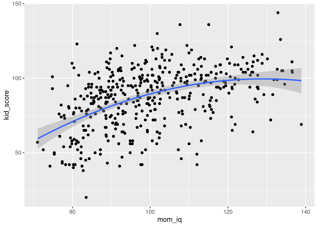
- Based on the results of the preceding two parts, is there any evidence that the slope of the predictive relationship between
kid_scoreandmom_iqvaries withmom_iq?
Yes: the estimated coefficient on mom_iq^2 is highly statistically significant, and from the plot we see that there is a "practically significant" amount of curvature in the predictive relationship.
- Suppose we wanted to run a regression of
kid_scoreonmom_iq,mom_hs, and their interaction. Write down three different ways of specifying this regression using R's formula syntax.
kid_score ~ mom_iq + mom_hs + mom_iq:mom_hskid_score ~ mom_iq * mom_hskid_score ~ (mom_iq + mom_hs)^2
- Run a regression of
kid_scoreonmom_hs,mom_iqand their interaction. Display a tidy summary of the estimates, standard errors, etc. Is there any evidence that the predictive relationship betweenkid_scoreandmom_iqvaries depending on whether a given child's mother graduated from high school? Explain.
tidy(lm(kid_score ~ mom_iq * mom_hs, kids))## # A tibble: 4 × 5
## term estimate std.error statistic p.value
## <chr> <dbl> <dbl> <dbl> <dbl>
## 1 (Intercept) -11.5 13.8 -0.835 4.04e- 1
## 2 mom_iq 0.969 0.148 6.53 1.84e-10
## 3 mom_hs 51.3 15.3 3.34 9.02e- 4
## 4 mom_iq:mom_hs -0.484 0.162 -2.99 2.99e- 3Let's introduce a bit of notation to make things clearer. The regression specification is as follows:
\[
\texttt{kid_score} = \widehat{\alpha} + \widehat{\beta} \times \texttt{mom_hs} + \widehat{\gamma} \times \texttt{mom_iq} + \widehat{\delta} \times (\texttt{mom_hs} \times \texttt{mom_iq})
\]
Now, mom_hs is a dummy variable that equals 1 if a child's mother graduated from high school For a child whose mother did not graduate from high school, our prediction becomes
\[
\texttt{kid_score} = \widehat{\alpha} + \widehat{\gamma} \times \texttt{mom_iq}
\]
compared to the following for a child whose mother did graduate from high school:
\[
\texttt{kid_score} = (\widehat{\alpha} + \widehat{\beta}) + (\widehat{\gamma} + \widehat{\delta})\times \texttt{mom_iq}
\]
Thus, the coefficient \(\widehat{\delta}\) on the interaction mom_iq:mom_hs is the difference of slopes: high-school minus no high school. The point estimate is negative, large, and highly statistically significant. We have fairly strong evidence that the predictive relationship between kid_score and mom_iq is less steep for children whose mothers attended high school. For more discussion of this example, see this document.
If you're rusty on the F-test, this may help.↩︎